Update (21 May 18): It turns out this post is one of the top hits on google for “python travelling salesmen”! That means a lot of people who want to solve the travelling salesmen problem in python end up here. While I tried to do a good job explaining a simple algorithm for this, it was for a challenge to make a progam in 10 lines of code or fewer. That constraint means it’s definitely not the best code around for using for a demanding application, and not the best for learning to write good, readable code. On the other hand, it is simple and short, and I explain each line. So stick around if you’re up for that. Otherwise, while I haven’t used it myself, Google has a library “OR-Tools” that has a nice page about solving the travelling salesmen problem in python via their library. So maybe check that out!
Update (29 May 19): I wrote a small Julia package to exactly solve small TSP instances: https://github.com/ericphanson/TravelingSalesmanExact.jl.
A few weeks ago I got an email about a high performance computing course I had signed up for; the professor wanted all of the participants to send him the “most complicated” 10 line Python program they could, in order to gauge the level of the classAnd to submit 10 blank lines if we didn’t know any Python!"
.
I had an evening free and wanted to challenge myself a bit, and came up with the idea of trying to write an algorithm for approximating a solution to the traveling salesman problem. A long time ago, I had followed a tutorial for implementing a genetic algorithm in java for this and thought it was a lot of fun, so I tried a genetic algorithm first and quickly found it was hard to fit in ten lines. I changed to a simulated annealing approach and found a nice pedagogical tutorial here: theprojectspot.com//simulated_annealing (in java, however). I should mention: I don’t really know python, and haven’t done any non-tutorial-level programming in general. So I’m sure there’s a lot to improve here, and I hope the reader proceeds at their own risk.
Warnings aside, here’s the resultwhich has been fixed up a little since then
:
1 import random, numpy, math, copy, matplotlib.pyplot as plt
2 cities = [random.sample(range(100), 2) for x in range(15)];
3 tour = random.sample(range(15),15);
4 for temperature in numpy.logspace(0,5,num=100000)[::-1]:
5 [i,j] = sorted(random.sample(range(15),2));
6 newTour = tour[:i] + tour[j:j+1] + tour[i+1:j] + tour[i:i+1] + tour[j+1:];
7 if math.exp( ( sum([ math.sqrt(sum([(cities[tour[(k+1) % 15]][d] - cities[tour[k % 15]][d])**2 for d in [0,1] ])) for k in [j,j-1,i,i-1]]) - sum([math.sqrt(sum([(cities[newTour[(k+1) % 15]][d] - cities[newTour[k % 15]][d])**2 for d in [0,1] ])) for k in [j,j-1,i,i-1]])) / temperature) > random.random():
8 tour = copy.copy(newTour);
9 plt.plot([cities[tour[i % 15]][0] for i in range(16)], [cities[tour[i % 15]][1] for i in range(16)], 'xb-');
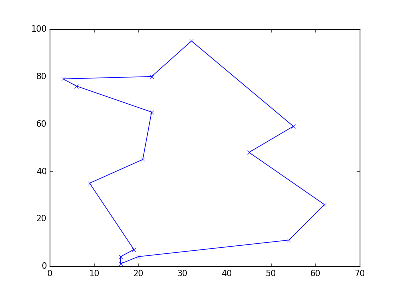
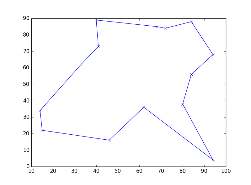
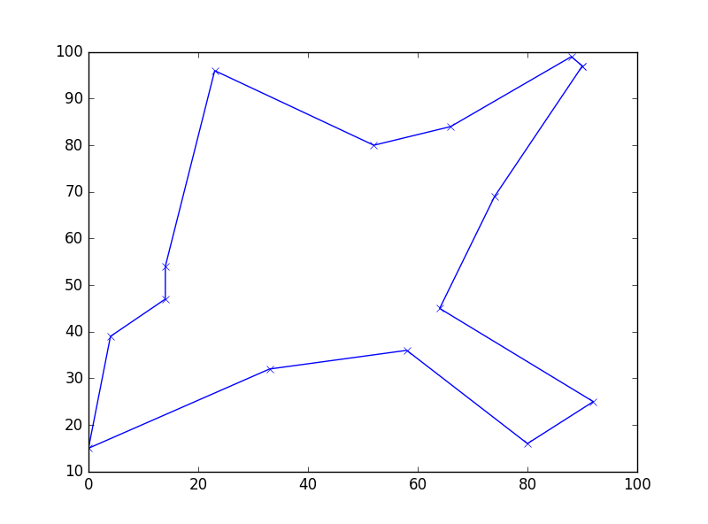
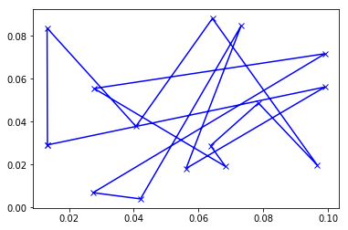
10 plt.show()which you can download here if you want. A few sample outputs:
Images generated by four consecutive runs of the python program.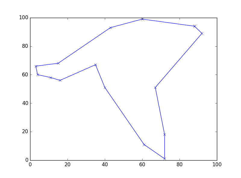
NoteThank you to Monish Kaul for pointing out this problem!
: if you’re using your own list of cities, it can help to rescale the coordinates so they run between 0 and a 100 by a simple affine transformation
xmin = min(pair[0] for pair in cities)
xmax = max(pair[0] for pair in cities)

ymin = min(pair[1] for pair in cities)
ymax = max(pair[1] for pair in cities)

def transform(pair):
    x = pair[0]
    y = pair[1]
    return [(x-xmin)*100/(xmax - xmin), (y-ymin)*100/(ymax - ymin)]

rescaled_cities = [ transform(b) for b in cities]
To illustrate, I generated some cities via
cities = [(random.random()/10, random.random()/10) for x in range(15)];which gives cities with coordinates between 0 and 0.01. Running the code with these cities gives a terrible result:
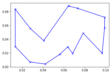
But if we run the code with rescaled_cities (and plot with the original coordinates), we find a much nicer result:
A line by line reading
As the professor mentioned in his reply, the code is completely unreadable. I thought it would be good to document it somewhere, and why not here.
1 import random, numpy, math, copy, matplotlib.pyplot as pltThis first line is just Python imports to use different commands.
2 cities = [random.sample(range(100), 2) for x in range(15)];The goal here is to make an list of “cities”, each which are simply a list of two coordinates, chosen as random integers from 0 to 100. I think a better practice usually would to make a constant for the grid size and the number of cities, and use that throughout the script. But with the 10 line requirement, all that will have to be hardcoded.
To explain the command itself, starting from the innermost command, range(100) returns the list [0,1,2,...,100]. Then random.sample( ,2) randomly chooses a set of size 2 from the list. This in fact makes it so that for each city, it’s first and second coordinates will never be the same. Since we just want to come up with some cities for the algorithm to run on, this doesn’t really matter; we could’ve hardcoded a list of cities here insteadI see them as allowing math-y set-like notation, but I’ll leave the explanation to the experts on the other side of the link. I’ll use them a lot to save space.
This last piece thus repeats the random sampling 15 times and forms a list of these pairs of coordinates, which I called cities.
3 tour = random.sample(range(15),15);A “tour” will just be a list of 15 numbers indicating an order to visit the cities. We’ll assume you need a closed loop, so the last city will be automatically connected to the first. Here we just choose a random order to start off with. Python also has a random.shuffle() command, but then we would need two lines: one to create a list, and another to shuffle it. By asking for a random sample of 15 numbers from a list of 15 elements, we get a shuffled list created for us in one line.
4 for temperature in numpy.logspace(0,5,num=100000)[::-1]:We start off a for-loop. In the tutorial I was reading (linked above), they do something like
while (temp > 1):
    ...
    temp *= 1 - coolingRate
and this was my attempt to write that in one line. I don’t actually really know why you want an exponentially decreasing temperature in a simulated annealing algorithmBriefly searching, I found this paper which might be relevant?
; I just followed the tutorial. The command numpy.logspace(0,5,num=100000) gives a list of 100,000 numbers between \(10^0\) and \(10^5\) so that the (base 10) logarithm of these numbers is evenly spaced. So choosing numbers in this alone should recover exponentially distributed temperatures. However, they are in lowest-first order. Since we want the temperature to start high, I added [::-1] which reverses the list.
5 [i,j] = sorted(random.sample(range(15),2));
6 newTour =  tour[:i] + tour[j:j+1] +  tour[i+1:j] + tour[i:i+1] + tour[j+1:];
I’ll group these two lines because together they do a single task which I had hoped to do in one line. The objective here is to make a new tour by randomly swapping two cities in tour. I do this by choosing two numbers i,j from the 15 possible cities via random.sample( ,2) as before (now glad that the two numbers will be distinct), and then order them via sorted( ). Then I piece together the new tour manually, by copying the old tour until (but not including) index i, concatenating the jth city from the old tour, continuing copying the old tour until index j where we swap in the ith city, and finish with the rest of the old tour. These two lines bugged me alot
Allie Brosh, “The Alot is Better Than You at Everything,” Hyperbole and a Half (2010), hyperboleandahalf.
, because it seemed like an inelegant way swap two elements of the list, and because it needed two lines. Looking back now though, I don’t really mind it. Seems like the simple way to go.
7 if math.exp( ( sum([ math.sqrt(sum([(cities[tour[(k+1) % 15]][d] - cities[tour[k % 15]][d])**2 for d in [0,1] ])) for k in [j,j-1,i,i-1]]) - sum([ math.sqrt(sum([(cities[newTour[(k+1) % 15]][d] - cities[newTour[k % 15]][d])**2 for d in [0,1] ])) for k in [j,j-1,i,i-1]])) / temperature) > random.random():
8   tour = copy.copy(newTour);
This one is terribly long, but only because I skipped using variables to save a few lines. If we define
oldDistances =  sum([ math.sqrt(sum([(cities[tour[(k+1) % 15]][d] - cities[tour[k % 15]][d])**2 for d in [0,1] ])) for k in [j,j-1,i,i-1]]
newDistances =  sum([ math.sqrt(sum([(cities[newTour[(k+1) % 15]][d] - cities[newTour[k % 15]][d])**2 for d in [0,1] ])) for k in [j,j-1,i,i-1]]))
then the code becomes a lot cleaner:
7 if math.exp( ( oldDistances - newDistances) / temperature) > random.random():
8   tour = copy.copy(newTour);
which is a little easier to understand. First, if we accept the condition on the if statement, we will update our old tour to this new tour. The idea is that in the metaphor with statistical mechanics, the sum of the distances between all the cities is the energy of the system, which we wish to minimize. We consider the Gibbs factor \(\mathrm{e}^{-\Delta E / T}\) of the exponential of the (negative) change in energy over temperature which should be something like the probability of transitioning to the new state from the old one. I only sum the distances from and to the ith and jth cities, because the rest of the distances are the same for the two tours and will cancel. If this factor has \(\mathrm{e}^{-\Delta E / T}>1\) then the new energy is lower, and we should definitely take the new tour. Otherwise, even if it’s worse, we want to take the new tour with some probability so that we don’t get stuck in a local minimum. We will choose it with probability \(\mathrm{e}^{-\Delta E / T}\) by choosing a uniformly random number in \(r \in [0,1]\) by Python’s random.random() and asking for \(\mathrm{e}^{-\Delta E / T} > r\). This was a little confusing to me at first, but if I just think of \(\mathrm{e}^{-\Delta E / T} = \frac{3}{4}\), then we accept as long as \(\frac{3}{4}\) is larger than our uniformly random number, which should happen \(\frac{3}{4}\) of the timeYes, somehow this convinces me when the same formula with a variable did not.
.
We actually finish the algorithm here. We choose to update our tour or not as described above, lower the temperature, randomly swap two cities, and try again until we run out of temperatures (here, I put 100,000 of them). At the end, whatever is in the variable tour is our best guess as to the optimal route. I have no idea how to figure out analytically any type of convergence result or confidence in this output. This is partly why we have the next two linesThanks to Vincent for suggesting an improvement in line 9!
.
9  plt.plot([cities[tour[i % 15]][0] for i in range(16)], [cities[tour[i % 15]][1] for i in range(16)], 'xb-');
10 plt.show()
In these two lines, the Python module matplotlib plots the cities and connects them according to our best guess tour. I’m pretty impressed that it’s a two line problem! The pictures are nice, and for a small number of cities, fairly convincing to the eye that it’s at least a pretty good route. That is, the algorithm did something! Considering that we used \(10^5\) loop iterations and a brute force solution of searching over all possible \(15! \sim 10^{12}\) tours would take much longer (though would be guaranteed to be optimal), I’m happy with the resultHappy, though perhaps not content: of course, I want something better than “it looks pretty good”
. As for the code itself, we just have to get everything in order. First, the list comprehension
[cities[tour[i % 15]] for i in range(16) ]writes out the cities in order according to the tour, and includes the first one again at the end (using that % in Python is modulo). Then we select for the first or second coordinate by adding a [0] or [1] index:
[cities[tour[i % 15]][0] for i in range(16) ]The string 'xb-' tells matplotpy to draw x’s on the points, and connect them with blue lines. Lastly, the command plt.plot( ) generates this plot, and plt.show() displays it.
And that’s it!
In retrospect, I think simulated annealing was a good fit for the ten line constraint. Looking at the code, lines 1-3 are just mandatory import statements and choosing an instance of TSM to solve. Lines 4-8 are the whole algorithm, and it is almost a transcription of pseudocode. In the tutorial actually, they save the best route as they go, because sometimes it’s better than the last route, and there’s basically no cost to doing so in that context. I drop that here to save space, but for a small amount of cities and large number of temperatures, it still works out fine. I originally submitted the code with ten cities and 10,000 temperatures, and the professor told me that it was quite fast, even compared to lengthier implementations. I think that may be an artifact of the small number of cities, and that the code probably doesn’t scale as well. At ten cities the speed up over brute force is only \(10! \sim 10^6\) versus \(10^4\) loops, so it becomes much more impressive at the fifteen city mark. On my computer it still only takes a few seconds for the \(10^5\) loops, but of course it takes about ten times longer for each additional number in that exponent, so it’s not really feasible to check the scaling much past fifteen citiesand with more cities, it becomes harder to see by eye how good or bad the final route is.
.
Going forward, it would be interesting to try to learn about estimating the optimality of the results of such an algorithm, and more about the choice of temperature schedule. I’m not sure I will any time soon though. Another interesting thing would be trying to write a parallel version, maybe for a GPU. Since the size of the solution space grows factorially with the number of cities, I think there should be a big regime where it’s feasible to store all of the cities on each computational node yet have too many cities to find even an approximate solution in a reasonable amount of time with a single node.
The algorithm I implemented here has a global temperature and current route, and each iteration of the loop needs the result of the one before it. But that doesn’t really seem essential. Each node could run it’s own copy of the algorithm (with it’s own temperature and current route), and just broadcast it’s best-yet route to all (or just some of) the other nodes every so often. Each node could then just adopt the best route they receive as their current route, and continue iterating from there. Since we are trying to iterate towards the optimal solution by random swaps in this huge solution space, the likelihood of two nodes duplicating work should be very low, so this method could provide a decent speed-up. I’m not sure how the scaling with the number of nodes would be, however. Anyway, I’m sure all of this is old territory in the optimization world. Lots to learn.