Landauer's Principle and the balance equation

I’ve been working on my thesisEdit: this was my master’s thesis

over reading week, and I think I’ve finished my introduction to Landauer’s Principle. I ended up writing a pretty detailed derivation of the balance equation, and thus Landauer’s bound, so I thought it might be useful to post here.

Landauer's principle states that there is a minimal energetic cost for a state transformation \(\rho^\text{i}\to \rho^\text{f}\) on a system \(\mathcal{S}\) via the action of a thermal reservoir \(\mathcal{E}\) at temperature \((k_B\beta)^{-1}\)⊕ \(k_B \approx 1.38 \times 10^{-23}\) Joules per Kelvin is Boltzmann's constant.

. In particular, if \(\Delta S_\mathcal{S}\) is the change of entropy of the system \(\mathcal{S}\), and \(\Delta Q_\mathcal{E}\) is the change in energy of the reservoir \(\mathcal{E}\), then \[ \Delta Q_\mathcal{E}\geq \beta^{-1}\Delta S_\mathcal{S}. \qquad(1)\] This principle has generated interest since its inception in 1961; see [Section 1, RW14]⊕ [RW14]: An improved Landauer Principle with finite-size corrections, D. Reeb and M. Wolf, 2014 (v3).

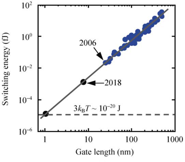
for a recent summary. First, the bound has allusions to practicality: perhaps the energy efficiency of our computers will be limited. For changing the state of a classical or quantum bit however, the bound is at most \[ \Delta Q_\mathcal{E}\geq k_B\cdot T \log 2 \approx (9.6 \times 10^{-24} J/K)\cdot \] which is extremely small for reasonable temperatures \(T\); yet, modern processors are within several orders of magnitude of this limit, as shown in Figure 1.

Energy cost of changing state for modern silicon transistors, as compared to a theoretical minimum for classical bits encoded in electron charge at room temperature. Figure reproduced from Figure 1(a) of Energy dissipation and transport in nanoscale devices by Eric Pop (2010).

Moreover, in 1973 Bennett showed that any Turing machine program may be implemented in a reversible manner, so that \(\Delta S_\mathcal{S}=0\). Reversible computing is an area of considerable practical interest and continuing theoretical work.

More fundamentally, Landauer's bound is a direct relationship between energy and information (entropy).⊕ From now on, we will use natural units so that \(k_B=\hbar=1\).

In fact, Landauer's principle follows from the entropy balance equation \[ \Delta S_\mathcal{S}+ \sigma = \beta \Delta Q_\mathcal{E} \qquad(2)\] where \(\sigma\) is the entropy production.

We will define \(\sigma\) and prove (eq. 2), in a finite dimensional quantum unitary setup, following [Section 3, RW14] and [JP14]⊕ [JP14]: A note on the Landauer principle in quantum statistical mechanics, V. Jaksic and C. Pillet, 2014 (v1).

. We assume the system \(\mathcal{S}\) is described by a finite dimensional Hilbert space \(\mathcal{H}_\mathcal{S}\), with self-adjoint Hamiltonian \(h_{\mathcal{S}}\). The initial state on the system is given by a density matrixnon-negative trace-one operator on \(\mathcal{H}_\mathcal{S}\)

\(\rho^\text{i}\). Likewise, we assume the environment is described by a finite dimensional Hilbert space \(\mathcal{H}_\mathcal{E}\) with self-adjoint Hamiltonian \(h_{\mathcal{E}}\), and initial state \[ \xi^\text{i}= \frac{\exp(-\beta h_{\mathcal{E}})}{\operatorname{tr}(\exp(-\beta h_{\mathcal{E}}))} \qquad(3)\] the Gibbs stateGibbs states on \(\mathcal{E}\) are invariant under the free dynamics \(h_{\mathcal{E}}\); in this finite dimensional context, they are uniquely so. They thus have the interpretation of thermal equilibrium states.

at temperature \(\beta^{-1}\). The system and environment start uncoupled, so the joint initial state is \(\rho^\text{i}\otimes \xi^\text{i}\). The evolution of the joint system is given by a unitary operator \(U \in \mathcal{B}(\mathcal{H}_\mathcal{S}\otimes \mathcal{H}_\mathcal{E})\), leading to the final joint state \(U\rho^\text{i}\otimes \xi^\text{i}U^*\). We decouple the systems, yielding \[ \begin{aligned} \rho^\text{f}= \operatorname{tr}_\mathcal{E}(U \rho^\text{i}\otimes \xi^\text{i}U^*), \qquad \xi^\text{f}= \operatorname{tr}_\mathcal{S}(U\rho^\text{i}\otimes \xi^\text{i}U^*) \end{aligned} \] as the final state on the system, environment, respectively.

We identify two quantities of interest during this process: \(\Delta S_\mathcal{S}\), the change of entropy of the system of interest, and \(\Delta Q_\mathcal{E}\), the change of energy of the environment, defined as⊕ Note the sign convention.

\[ \begin{aligned} \Delta S_\mathcal{S}:\!&= S(\rho^\text{i}) - S(\rho^\text{f}), & \Delta Q_\mathcal{E}:\!&= \operatorname{tr}(h_{\mathcal{E}}\xi^\text{f})- \operatorname{tr}(h_{\mathcal{E}}\xi^\text{i}), \end{aligned} \] where \(S(\rho) := - \operatorname{tr}\rho\log\rho\) is the von Neumann entropy. Recall the relative entropy \(S(\eta|\nu) = \operatorname{tr}(\eta\log\eta-\log \nu))\) of two faithful states \(\eta\) and \(\nu\) has \(S(\eta|\nu)\geq 0\) with equality if and only if \(\eta=\nu\).⊕ See sections 2.5-2.6 of Entropic Fluctuations in Quantum Statistical Mechanics. An Introduction by Jaksic et al (2011) for a review of entropy functions in finite dimensional quantum mechanics.

With this function, we define the entropy production \[ \sigma := S(U \rho^\text{i}\otimes \xi^\text{i}\,U^* | \rho^\text{f}\otimes \xi^\text{i}). \] By definition of relative entropy, the entropy production may be written \[\begin{aligned} \sigma = \operatorname{tr}\big(U \rho^\text{i}\otimes \xi^\text{i}U^* \, \log (U \rho^\text{i}\otimes \xi^\text{i}U^*)\big) -\operatorname{tr}\big(U \rho^\text{i}\otimes \xi^\text{i}U^* \, \log(\rho^\text{f}\otimes \xi^\text{i})\big). \end{aligned}\] We then recognize the first term as an entropy, and expand the second term using the following claim.

This yields

\[\begin{aligned}\sigma &= - S(U \rho^\text{i}\otimes \xi^\text{i}U^*) - \operatorname{tr}\big( U \rho^\text{i}\otimes \xi^\text{i}U^* \, (\log \rho^\text{f}\otimes \operatorname{id})\big) \\&\qquad- \operatorname{tr}\big( U \rho^\text{i}\otimes \xi^\text{i}U^* \, ( \operatorname{id}\otimes \log \xi^\text{i})\big).\end{aligned}\]

Since entropy is invariant under a unitary transformationAs may immediately be seen by the spectral theorem: if \(\rho\) has spectral decomposition \(\rho = \sum_i \mu_i P_i\), then \(S(\rho) = -\sum_i \mu_i\log \mu_i= S(U\rho U^*)\), since eigenvalues are invariant under unitary transformations (change of basis).

, we have \(S(U \rho^\text{i}\otimes \xi^\text{i}U^*) = S(\rho^\text{i}\otimes \xi^\text{i})\). Furthermore, by definition of the partial trace, \[\begin{aligned}\operatorname{tr}\big( U \rho^\text{i}\otimes \xi^\text{i}U^* \, (\log \rho^\text{f}\otimes \operatorname{id})\big) = \operatorname{tr}\big(\operatorname{tr}_\mathcal{S}(U \rho^\text{i}\otimes \xi^\text{i}U^*) \log \rho^\text{f}\big),\end{aligned}\] which is simply \(\operatorname{tr}(\rho^\text{f}\log \rho^\text{f}) = -S(\rho^\text{f})\). Using this argument for the third term as well, we are left with \[\begin{aligned}\sigma =-S(\rho^\text{i}\otimes \xi^\text{i}) + S(\rho^\text{f}) - \operatorname{tr}(\xi^\text{f}\log \xi^\text{i}).\end{aligned}\] But \[\begin{aligned}S(\rho^\text{i}\otimes \xi^\text{i}) &= -\operatorname{tr}\big(\rho^\text{i}\otimes \xi^\text{i}\log(\rho^\text{i}\otimes \xi^\text{i}) \big) \\&= -\operatorname{tr}\big(\rho^\text{i}\otimes \xi^\text{i}(\log\rho^\text{i}\otimes \operatorname{id})\big) - \operatorname{tr}\big(\rho^\text{i}\otimes \xi^\text{i}(\operatorname{id}\otimes\log \xi^\text{i})\big)\\&=-\operatorname{tr}\big(\rho^\text{i}\log\rho^\text{i}\otimes \xi^\text{i}\big) - \operatorname{tr}\big(\rho^\text{i}\otimes \xi^\text{i}\log \xi^\text{i}\big) \\&=- \operatorname{tr}(\rho^\text{i}\log \rho^\text{i}) \operatorname{tr}(\xi^\text{i}) - \operatorname{tr}(\xi^\text{i}\log \xi^\text{i}) \operatorname{tr}(\rho^\text{i})\\&= S(\rho^\text{i}) + S(\xi^\text{i}),\end{aligned}\] using that \(\operatorname{tr}(\rho^\text{i}) = \operatorname{tr}(\xi^\text{i})=1\). Then, \[\begin{aligned}\sigma &= -S(\rho^\text{i}) +S(\rho^\text{f})- S(\xi^\text{i}) - \operatorname{tr}(\xi^\text{f}\log \xi^\text{i}) \\&= -\Delta S_\mathcal{S}- \operatorname{tr}\big((\xi^\text{f}- \xi^\text{i}) \log \xi^\text{i}\big).\end{aligned}\] Additionally, using (eq. 3), \[\begin{aligned}\log \xi^\text{i}= -\beta h_{\mathcal{E}}- \log(\operatorname{tr}(\exp(-\beta h_{\mathcal{E}})),\end{aligned}\] so \[\begin{aligned}\sigma &= -\Delta S_\mathcal{S}+ \beta\operatorname{tr}\big((\xi^\text{f}- \xi^\text{i}) h_{\mathcal{E}}\big) + \log(\operatorname{tr}(\exp(-\beta h_{\mathcal{E}})))\operatorname{tr}(\xi^\text{f}- \xi^\text{i}) \\&= -\Delta S_\mathcal{S}+ \beta \Delta Q_\mathcal{E},\end{aligned}\] using that \(\operatorname{tr}(\xi^\text{f}- \xi^\text{i}) = 1-1=0\).

We thus have the balance equation (eq. 2). Landauer’s Principle (eq. 1) follows by simply noting \(\sigma\geq 0\) as it is a relative entropy.

We may interpret (eq. 2) as a microscopic Clausius formulation of the Second Law of Thermodynamics [BHN+14]⊕ [BHN+14]: The second laws of quantum thermodynamics F. Brandao et al, 2013 (v4).

. More specifically, we may interpret \(\beta \Delta Q_\mathcal{E}=\int_\text{i}^\text{f}\frac{\mathrm{d} Q_\mathcal{E}}{T}= \Delta S_\mathcal{E}^\text{Clausius}\) as the Clausius entropy change of the environment.⊕ Note: We’re making an analogy to the Clausius formulation of the Second Law of Thermodynamics, but not a formal relationship. The balance equation presented here and the 2nd law are part of two different frameworks.

Then, with a minus sign to account for our sign convention, we will interpret \(\Delta S_\mathcal{S}^\text{Clausius} =-\Delta S_\mathcal{S}\), and the Second Law is \[\begin{aligned}\Delta S^\text{Clausius}_\mathcal{E}+\Delta S^\text{Clausius}_\mathcal{S}=\text{entropy production}\geq 0.\end{aligned}\] In this language then, \(\sigma\) serves as the entropy production, which gives it its name. The classical Second Law, however, is a statement about macroscopic quantities obtained from the behavior of \(\gtrsim 10^{23}\) particles. Within the theory of quantum mechanics and our assumptions, however, the balance equation (eq. 2) is exact on a microscopic level.