When do we lose correlations under Markovian evolution?

Loss to the environment

After letting the joint system evolve for some time, we close the divided gap. At this point, the system is “frozen” and the particles can no longer jump between boxes. However, it is still perfectly correlated; if there are \(n\) particles on the left, there are exactly \(N-n\) on the right.

Now, we will consider what happens to those correlations if we let the left side of the box interact with some kind of environment. We will consider three types of interactions, showing qualitatively different behavior, starting with a very simple model.

What happens if we just open a door and let the particles go? In this model, at each time step, one particle leaves the left side of the box and escapes to the environment, until they are all gone.

We can see that after at most \(N\) timesteps, all the particles are gone from the left, no matter how many particles were originally on the left side. In particular, the joint distribution becomes \(\delta _0 \otimes p\) for \(p = \frac{1}{2^N}\sum_{n=0}^N{N \choose n} \delta _{N-n}\), a product state, reflecting the complete loss of correlations. We can see how this evolution changes the joint distribution.

We see that the joint distribution soon has no “diagonal” pieces left, which correspond to correlations between the two systems. We also notice the marginal distribution of particles on the right remains invariant, as it should; we are only evolving the left side.

Now, let’s consider a different model of evolution on the left side of the box. Let us assume that the particles begin to undergo a birth and death process, where at each timestep, with probability \(\frac{1}{10}\), a new particle is born, with probability \(\frac{1}{10}\), a particle dies, and with probability \(\frac{8}{10}\), nothing happens. We cap the population at 20; if there are 20 particles on the left, then the probability of birth is zero, and the probability of nothing happening is increased to \(\frac{9}{10}\), and likewise, if there are no particles on the left, then the probability of death is zero, and that of nothing happening is \(\frac{9}{10}\).

We can see what this looks like on the particle level in the following animation.

We can also see what happens to the joint distribution (which we assume is initially \(\pi\) defined above).

⊕ This animation would be too slow if it were run at 1 timestep per frame like the others, so instead it’s 10 timesteps per frame for a total of 600 timesteps.

We see the joint distribution “smears out” to a flat line. That is, the joint distribution converges asymptotically to \(u \otimes p\) where \(u\) is uniform, and \(p\) is the distribution defined previously. So we see again that this evolution causes a loss of correlations between the two subsystems: as time goes on, knowing how many particles are on the left tells us less and less about how many particles are on the right. But this time it actually takes infinite time to lose all the correlationsthat is, until the joint distribution is just the product of its marginals

.

In fact, both of the evolutions above have a particular property that guarantees this asymptotic loss of correlations: they are irreducible and aperiodic Markov chains (on the left system alone). Here, irreducible means that if there are \(n\) particles on the left, then for any \(n'\), there is some probability of there being \(n'\) particles on the left at some later point in time. Aperiodic means that that the period of the Markov chain is 1, where the period is defined as \[ \operatorname{gcd}\{ m : \Pr[X_m = i | X_0 = i] > 0 \} \] where \(X_m\) is the random variable representing how many particles there are on the left at step \(m\).

It turns out that any irreducible and aperiodic Markov chain has a unique invariant distribution, and any initial distribution will asymptotically converge to that distribution. This implies an asymptotic loss of correlations, as follows. Let \(P\) be the transition matrix of an irreducible and aperiodic Markov chain acting on the left box only. Then, recalling our initial joint distribution is \[ \pi = \frac{1}{2^N}\sum_{n=0}^N{N \choose n} (\delta _n \otimes \delta _{N-n}), \] then the joint distribution after \(k\) steps of the Markov chain is given by \[ \pi ( P^k \otimes \operatorname{id}) = \frac{1}{2^N}\sum_{n=0}^N{N \choose n} ( (\delta _n P^k) \otimes \delta _{N-n}). \] But for any distribution \(\mu\), we have \(\mu P^k \to q\) as \(k\to\infty\), where \(q\) is the stationary distribution of the Markov chain. Thus, \[ \pi ( P^k \otimes \operatorname{id}) \rightarrow \frac{1}{2^N}\sum_{n=0}^N{N \choose n} ( q \otimes \delta _{N-n}) = q \otimes p \] and we find that the joint distribution becomes asymptotically uncorrelated.

But we don’t always lose correlations!

Let us instead choose our Markov dynamics on the left side of the box to be periodic. We will choose a simple process: at each step, the number of particles on the left increases by \(1\), unless it is at \(20\), at which point it resets to \(0\). This may seem like a strange kind of dynamics for particles in a box, but we could instead reinterpret “number of particles” as a position on a circular track, or something like that. Let’s see how it looks.

As promised, the number of particles simply loops around. Now, if we look away and look back, it might seem like the number of particles on the left is just some random number between \(0\) and \(20\), and is unrelated to the number of particles on the right. But in fact, since our dynamics is actually deterministic, if we simply keep track of the number of timesteps since the start of the evolution, we can figure out exactly the number of particles on the left at the start, and hence figure out how many particles on the right. We can see this reflected in how the joint distribution evolves.

We see that rather smearing to a horizontal, like in the birth death process, or becoming completely vertical, like in the simple loss example at the start, the distribution just cycles around, with those perfect correlations intact.

Summary (classical case)

Let us summarize what we’ve seen so far.

1. If we let one part of a joint system evolve independently, the two may decouple.

2. That decoupling can take infinitely long
   

3. Under periodic evolution, the joint system may not decouple.
   

Classical \(\textcolor{purple}{\Rrightarrow}\) quantum

Let us take out our classical-to-quantum dictionary (\(\textcolor{purple}{\Rrightarrow}\)), and find analogous quantities in the quantum case to those we have been studying. This will be an abridged translation; please see some of the references, e.g. (Wilde 2017; Nielsen and Chuang 2009; Avron and Kenneth 2019; Aubrun and Szarek 2017; Watrous 2018; Wolf 2018) at the end for more details about quantum information theory.

• Probability distributions \(p \in \mathbb{R}^d\) \(\textcolor{purple}{\Rrightarrow}\) quantum states \(\rho \in M_{d\times d}\).
  • \(p_i \ge 0 \textcolor{purple}{\Rrightarrow}\rho \succeq 0\),⊕ here, \(\succeq 0\) refers to positive semi-definite.
    
    
  • \(\sum _i p_i = 1 \textcolor{purple}{\Rrightarrow}\operatorname{tr}[\rho ] = 1\).
• Markov transition matrix \(P\) \(\textcolor{purple}{\Rrightarrow}\) \(\Phi\) linear, completely positive, trace-preserving map called a quantum channel.
  • \(P\) maps \(\mathbb{R}^d\) to \(\mathbb{R}^d\) \(\textcolor{purple}{\Rrightarrow}\) \(\Phi\) maps \(M_{d\times d}\) to \(M_{d\times d}\)
• Joint distribution \(\sum_i \lambda_i p_i \otimes q_i\) (convex combination of product distribution) \(\textcolor{purple}{\Rrightarrow}\) joint state \(\rho \in M_{d\times d} \otimes M_{d\times d}\).
  • Key difference: it’s possible that \(\rho \in M_{d\times d} \otimes M_{d\times d}\) cannot be expressed as \(\sum_i \lambda_i \rho _i \otimes \sigma _i\) for any \(\rho _i \succeq 0\) and \(\sigma _i \succeq 0\), probability distribution \(\{\lambda_i\}\). Entanglement!

Let us take a bit of a closer look at entanglement. It is a non-classical correlation between the two systems, and it’s a bit of a strange thing. It is “no-signalling”: you cannot use entanglement alone to send messages. On the other hand, it can help send messages, via a protocol called “superdense coding”: one can communicate \(2n\) bits of classical information by only transmitting \(n\) bits of data, using \(n\) pre-shared “bits of entanglement”\(n\) pairs of entangled qubits

. Before looking a bit more at what one can do with entanglement, let us consider: what states are entangled?

To get a feeling for this, let us consider the following 3D cross section of two-qubit quantum states, reproduced from (Avron and Kenneth 2019).

In this figure, the green part corresponds to all quantum states (within this 3D cross section); the blue part corresponds to “classical” (i.e. non-entangled) states, and hence the region inside the green part and outside of the blue part corresponds to the entangled states.

The magic square game

To get a better understanding of what one can do with the strange correlations given by entanglement, let us consider the (Mermin-Peres) Magic Square Game. This is a cooperative game, played by two players Alice and Bob, who play against a referee. The two players can agree on a strategy ahead of time, but then are isolated and can no longer communicate. The aim of the two players is to construct a magic square. This is a \(3\times 3\) grid of \(+1\)’s and \(-1\)’s such that the rows have an even number of \(-1\)’s and the columns have an odd number of \(-1\)’s.

It’s a magic square, because it’s impossible to construct such a thing. We can see this because if such a square existed, we could multiply all the elements together by first multiplying down the columns (getting a product of \(-1\) for each column), and then multiply those three values together, getting a \(-1\) overall for the product of all the elements. On the other hand, if we multiply across each row, we find each row has a product of \(+1\), which then multiplied together yields an overall product of \(+1\). Since the product has to be the same no matter the order we multiply in, such a square cannot exist!

⊕ Click me!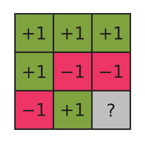

And yet, Alice and Bob claim to have constructed one. The referee will then give them a test to try to test that claim. The referee will ask Alice for one specific row, and Bob for one specific column (e.g. top row, second column). Alice and Bob pass the test if Alice’s row has an even number of \(-1\)’s, and Bob’s column an odd number, and they agree on the value (\(+1\) or \(-1\)) of the one square in the intersection of their row and column.

It’s a bit of a weak test (if the referee wanted to be really stringent, he or she would simply ask for all the entries), but it’s still impossible to pass 100% of the time when Alice and Bob only have access to classical mechanics. Essentially, the best they can do is agree ahead of time on a square like the one pictured, and hope the referee never asks about the “?” square. They will win \(8/9\) of the time this way (assuming the referee asks for rows and columns uniformly at random), but cannot win with probability \(1\)Note that neither Alice nor Bob knows where the intersection will be when asked for their row or column!

.

It turns out, however, that if Alice and Bob have access to pre-shared entanglement, and can each perform measurements of their shared entangled state, they can win every time!See, e.g. wikipedia for more details on how they can accomplish this.

If the referee only knew classical mechanics, after enough trials which the players pass each time, the referee might be convinced that Alice and Bob really did have a magic square! After all, classically the probability of them passing the test \(n\) times in a row is exponentially small: \((8/9)^n\).

How do we lose quantum entanglement?

Now that we’ve seen some of the power of entanglement as a correlation, let’s return to our original subject of study: the loss of correlations due to Markovian evolution on one part of a joint system.

It turns out one can formulate an analog to the irreducibility and aperiodicity of Markov chains, usually called primitivity. If \(\Phi\) is a primitive quantum channel, we have the same kind of convergence result as in the aperiodic and irreducible classical case: \(\Phi^n(\rho) \rightarrow \sigma\) as \(n\to\infty\) for any initial state \(\rho\). Then, just like in the classical case, this gives convergence of the joint state to a product state (here, to \(\sigma \otimes I/d\) where \(I\) is the identity matrix and \(d\) the dimension; \(I/d\) is analogous to a uniform distribution). It turns out that product states of full support are in the interior of the set of separable states (non-entangled states) is interior of the set of all statesAs shown in (Lami and Giovannetti 2016), using a fundamental result of (Gurvits and Barnum 2002) (strengthened to a quantitative bound in (Hanson, Rouzé, and França 2019)).

. Then the convergence \(\Phi ^n(\rho ) \rightarrow \sigma\) gives that there is a finite time for any joint state to become separable under this evolution.

What other kinds of evolutions destroy all entanglement in finite time? It turns out there’s a short list!

• Primitive quantum channels

• Direct sums thereof

• Any quantum channel such that after some number of iterations, it is a direct sum of primitive maps.

• That’s it!\(^*\)

\(*\): under a faithfulness assumption, namely that there exists an invariant state with full support (which is possibly non-unique).

This is the content of Proposition 3.11 of (Hanson, Rouzé, and França 2019), which is joint work with my collaborators Cambyse Rouzé and Daniel Stilck França. In fact, the “some number of iterations” above is one specific number, described in more detail in that proposition. We also consider the continuous time case, make connections to the so-called PPT\(^2\) conjecture, and establish explicit bounds on the number of iterations for a quantum channel to be entanglement-breaking, so I encourage you to click through to the preprint if you are interested.

References

Aubrun, Guillaume, and Stanisław J. Szarek. 2017. Alice and Bob Meet Banach: The Interface of Asymptotic Geometric Analysis and Quantum Information Theory. Mathematical Surveys and Monographs, volume 223. Providence, Rhode Island: American Mathematical Society.
Avron, Joseph, and Oded Kenneth. 2019. “An Elementary Introduction to the Geometry of Quantum States with a Picture Book.” http://arxiv.org/abs/1901.06688.
Gurvits, Leonid, and Howard Barnum. 2002. “Largest Separable Balls Around the Maximally Mixed Bipartite Quantum State.” Physical Review A 66 (6). https://doi.org/10.1103/PhysRevA.66.062311.
Hanson, Eric P., Cambyse Rouzé, and Daniel Stilck França. 2019. “On Entanglement Breaking Times for Quantum Markovian Evolutions and the PPT-Squared Conjecture.” arXiv:1902.08173 [Quant-Ph], February. http://arxiv.org/abs/1902.08173.
Lami, L., and V. Giovannetti. 2016. “Entanglement-Saving Channels.” Journal of Mathematical Physics 57 (3): 032201. https://doi.org/10.1063/1.4942495.
Nielsen, Michael A., and Isaac L. Chuang. 2009. Quantum Computation and Quantum Information. Cambridge University Press. https://doi.org/10.1017/cbo9780511976667.
Watrous, John. 2018. The Theory of Quantum Information. 1st ed. Cambridge University Press. https://doi.org/10.1017/9781316848142.
Wilde, Mark M. 2017. From Classical to Quantum Shannon Theory. http://arxiv.org/abs/1106.1445.
Wolf, Michael. 2018. “Quantum Channels & Operations Guided Tour.” https://www-m5.ma.tum.de/foswiki/pub/M5/Allgemeines/MichaelWolf/QChannelLecture.pdf.